Bloom Filters

API⌗

bf.add(x): adds x in the data structure
x in bf: tests if x is in the data structure.

Why not use Set or Dict?⌗

Bloom filters are more space efficients. They take memory lesser than the keys themselves.

Cons⌗

can’t store associated data.
does not support deletions.
It is probabilistic data structure. That means, x in bf might have false positives. There are no false negatives.

Applications⌗

Spell checkers: (40 years ago) Add the dictionary into the filter. If the word is in the bloom filter, it is higly likely tobe correctly spelled word.
list of forbidden password. E.g., too common password.
Modern applications: Routers, a lot of packets incoming.

How does it work?⌗

we have a data set S of size |S|.
have an array of n bits.
$b = \frac{n}{|S|}$ bits per element.
have k hash functions.

import numpy as np

class BitArray:
    def __init__(self, n):
        self.array = np.zeros((n >> 3) + 1, dtype=np.uint8)
    
    def set(self, i):
        i, j = divmod(i, 8)
        self.array[i] = self.array[i] | (1 << j)
    
    def get(self, i):
        i, j = divmod(i, 8)
        return bool(self.array[i] & (1 << j))

import xxhash

def get_hashes_for_str(x, k):
    # Only h1 and h2 are computed afresh. Remaining hash 
    # functions are just linear combinations of h1 and h2.
    
    assert k > 1
    
    h1 = xxhash.xxh64_intdigest(x, seed=42)
    h2 = xxhash.xxh64_intdigest(x, seed=84)
    hashes = [h1, h2]
    
    for i in range(2, k):
        hashes.append(h1 + i*h2)
    return hashes

class BloomFilter:
    def __init__(self, n, k):
        self.array = BitArray(n)
        self.k = k
        self.n = n
        
    def add(self, key):
        for h in get_hashes_for_str(key, self.k):
            self.array.set(h % self.n)
            
    def __contains__(self, key):
        for h in get_hashes_for_str(key, self.k):
            if not self.array.get(h % self.n):
                return False
        return True

text = "correct incorrect".split()
bm = BloomFilter(10, 5)

for word in text:
    bm.add(word)

for word in text:
    assert word in bm

assert "notcorrect" not in bm

Analysis⌗

Trade off between erro rate and space required. Data structre will be useful when there is a sweetspot on the tradeoff curve.

Assumption: The hash functions are independent and they distribute the data uniformly.

Out of n bits, focus on a particular bit. What is the probability that it has been set?

It is probability of 1 minus it hasn’t been set by any of the |S| elements, for any of the k hash functions.

$p = 1 - (1 - \frac{1}{n})^{k|S|}$.

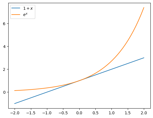
As can be seen by the plot below, $1+x$ can be approximated by $e^x$ when x is close to zero. In all cases, $e^x$ is an overestimate of $1+x$.

import matplotlib.pyplot as plt
x = np.linspace(-2, 2)
plt.plot(x, 1+x, label="$1 +x$")
plt.plot(x, np.exp(x), label="$e^x$")
plt.legend();

output image for above cell

<Figure size 640x480 with 1 Axes>

Thus, $p \approx 1 - e^{\frac{-k|S|}{n}} = 1 - e^{\frac{-k}{b}}$. Remember, b is the bits per element.

As $b \to \inf$, $p \to 0$.

Thus, the probability of false positive is $\epsilon = (1-e^{\frac{-k}{b}})^k$.

How to set K?⌗

Set K optimally. Fix the b, then set k to minimize the error. Using calculus, $k \approx (ln 2) b$.

When we plug this back into the p, we get $\epsilon \approx (\frac{1}{2})^\left((ln 2) b\right)$. Notice that error rate is exponential in b.

Using little bit of algebra we can get $b \approx 1.44 log_2{\frac{1}{\epsilon}}$. (Hint: $1.44 \approx \frac{1}{ln2}$.)

How does theory differ from practice⌗

import string
import random
import numpy as np

letters = np.array(list(string.ascii_letters + string.digits))

def random_str():
    return ''.join(np.random.choice(letters, np.random.randint(4, 9)))

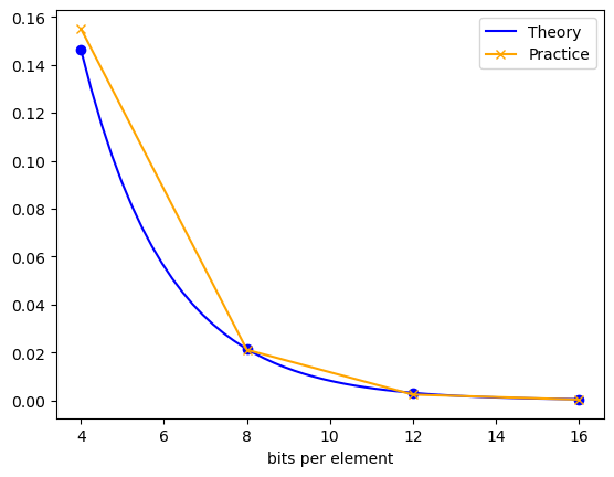
Generate 1M keys, and insert them in the bloom filter. Just for sanity check, I will test if there is no false negative. Then I will generate keys at random, check if it is in actually there, and how often does bloom filter give false positive. Recall that error rate as a function of b = n/10M is $\approx (\frac{1}{2})^\left((ln 2) b\right)$.

actually_there = set()
set_size = int(1e6)
while len(actually_there) != set_size:
    actually_there.add(random_str())

from tqdm.auto import tqdm

bs = [4, 8, 12, 16]
fpve_rate = []
theory = []

for b in bs:
    theory.append(.5**(np.log(2)*b))
    bm = BloomFilter(b*set_size, k=int(np.log(2)*b))
    for key in tqdm(actually_there, "Inserting"):
        bm.add(key)
    
    for key in tqdm(actually_there, "Sanity Checking"):
        assert key in bm
        
    fpve, total = 0, 0
    while total < 10_000:
        key = random_str()
        if key in actually_there: continue
        if key in bm:
            fpve += 1
        total += 1
    
    fpve_rate.append(fpve/total)

Inserting:   0%|          | 0/1000000 [00:00<?, ?it/s]

Sanity Checking:   0%|          | 0/1000000 [00:00<?, ?it/s]

Inserting:   0%|          | 0/1000000 [00:00<?, ?it/s]

Sanity Checking:   0%|          | 0/1000000 [00:00<?, ?it/s]

Inserting:   0%|          | 0/1000000 [00:00<?, ?it/s]

Sanity Checking:   0%|          | 0/1000000 [00:00<?, ?it/s]

Inserting:   0%|          | 0/1000000 [00:00<?, ?it/s]

Sanity Checking:   0%|          | 0/1000000 [00:00<?, ?it/s]

bs_lin = np.linspace(bs[0], bs[-1])
plt.plot(bs_lin, .5**(np.log(2)*bs_lin), label="Theory", c='b') 
plt.plot(bs, theory, 'o', c='b')
plt.plot(bs, fpve_rate, '-x', label="Practice", c='orange')
plt.legend();
plt.xlabel("bits per element")

Text(0.5, 0, 'bits per element')

output image for above cell

<Figure size 640x480 with 1 Axes>

fpve_rate

[0.1551, 0.0211, 0.0024, 0.0003]

at b=12, false positive rate is already less than 1%